`clustord` Ordinal Models

Louise McMillan

2025-05-28

TL:DR

The proportional-odds model is named "POM" in the clustord() model argument. It is the most commonly-used model for ordinal data analysis, and it is the simplest, in that it has the fewest parameters and a consistent pattern for all categories of the ordinal response variables.

The ordered stereotype model is named "OSM" in the clustord() model argument. Compared with the proportional-odds model, it has one additional parameter for every category/level of the ordinal response variable. These additional parameters, plus its non-cumulative structure, make it much more flexible. Use the OSM if you think that your ordinal data may be very heterogeneous in terms of the patterns of different categories of the response variables.

The $\texttt{phi}_k$ score parameters for the response categories $k$ indicate how much information is available in each response category. If $\texttt{phi}_k$ and $\texttt{phi}_{k+1}$ are very similar (within 0.1 of each other) then that indicates that response categories $k$ and $k+1$ do not provide much information about any clustering structure, which means you could simplify your data by combining those two response categories without having much effect on the results of the analysis.

You can also use the $\texttt{phi}_k$ scores from the OSM as a data-driven numerical encoding of your ordinal response categories that is better than simply numbering the categories $1, 2, \ldots, q$ and then carry out analysis using methods for numerical data, such as k-means (Lloyd, 1982 and MacQueen, 1967).

Introduction

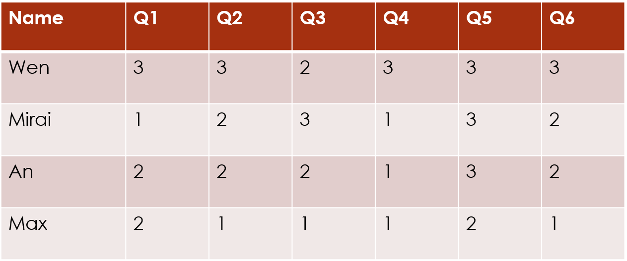
For this package, we assume that you have a dataset of ordinal data. The most common form of this is survey data, such as you might get by asking participants to ask a series of questions with Likert-scale answers (for example, ranking from 1 = “Strongly Disagree” to 5 = “Strongly Agree”).

We will refer to the data matrix as $\bm{Y}$. We index the rows of the data matrix with $i$ and the columns of the data matrix with $j$, so an individual response value is defined as $Y_{ij}$. The $q$ categories of each response variable $Y_{ij}$ are indexed with $k$, with $k = 1, \dots, q$.

There are three broad types of clustering: row clustering, column clustering and biclustering. Within each of these, there are multiple possible clustering structures. These are discussed in detail in the clustord Tutorial vignette, and summarised in the Clustering Structure Summary vignette.

If there are row clusters, they are indexed with $r$ and if there are column clusters they are indexed with $c$.

This vignette discusses the two types of ordinal models that are available in clustord: the proportional-odds model (POM) and the ordered stereotype model (OSM).

Proportional-odds model (POM)

The first model is the proportional-odds model (Agresti, 2000). This is the most widely-used ordinal model, and the simplest. The model is more easily recognisable as a regression model: $$\mbox{logit}P(Y \leq k \,|\, \bm{x}) = \log\left(\dfrac{P(Y \leq k \,|\, \bm{x})}{P(Y > k \,|\, \bm{x})}\right) = \mu_k - \bm{\beta}^T\bm{x} \; \; \mbox{for}\; k = 1, \dots, q-1$$ where $\mu_k$ is the intercept parameter for response category $k$ and $\bm{\beta}$ are the coefficients controlling the effect of $\bm{x}$ on the response, $Y$. The model is named “proportional-odds” because the coefficients do not depend on the response category, $k$. That is, the effect of $\bm{x}$ is the same for every single category of the response. Thus, the number of coefficients is only one more than the number of covariates.

This is also a cumulative ordinal model in that it is expressed as the probability of obtaining a given response category or lower, relative to the probability of getting any of the higher response categories. Along with the coefficients staying the same for all categories, this is the other part of how this model enforces similar patterns of effects for every response category.

The proportional-odds clustering forms in clustord were introduced in Matechou et al. (2016). Considering cell $(i,j)$ in the data matrix of responses, where if row $i$ is in row cluster $r$ and/or column $j$ is in column $c$ then the model has this general shape: $$\log\left(\dfrac{P(Y_{ij} \leq k \,|\, i \in r,\; j \in c)}{P(Y_{ij} > k \,|\, i \in r,\; j \in c)}\right) = \mu_k - \eta_{rcij} \; \; \mbox{for}\; k = 1, \dots, q-1$$ where $\mu_k$ is a parameter that controls the default probabilities of the different response categories in the absence of clustering, and $\eta_{rcij}$ is the remaining part of the linear predictor. $\eta_{rcij}$ is the part of the model that determines the clustering structure, and it is the same in both the proportional-odds model and the ordered stereotype model within clustord.

$\eta_{rcij}$ is subtracted from $\mu_k$, rather than added, so that if a parameter within $\eta_{rcij}$ is positive then that corresponds to a higher probability of obtaining higher response categories (whereas if it were added, positive effects would lead to a higher probability of obtaining lower response categories).

The logit notation above is the most compact way of expressing this model, but alternatively we can express it in terms of the probability, $\theta_{ijk}$, of getting a single response category, $k$, in cell $Y_{ij}$: $$\theta_{ijk} \,|\, i\in r,\;j \in c = \begin{cases} \dfrac{\exp(\mu_k - \eta_{rcij})}{1+\exp(\mu_k - \eta_{rcij})} & k = 1\\[10pt] \dfrac{\exp(\mu_k - \eta_{rcij})}{1+\exp(\mu_k - \eta_{rcij})} - \dfrac{\exp(\mu_{k-1} - \eta_{rcij})}{1+\exp(\mu_{k-1} - \eta_{rcij})} & 1 < k < q \\[10pt] 1 - \sum_{k=1}^{q-1} \theta_{ijk} & k = q \end{cases}$$

These are some of the potential clustering structures within clustord, expressed in POM form:

Column clustering and biclustering can similarly include covariates, in the same way as row clustering can. Note that because the coefficient/covariate structure of including covariates is the same in the clustering models regardless of whether the covariates are attached to the rows ($\bm{x}_i$) or the columns ($\bm{w}_j$), the clustord package combines their coefficients into one single cov parameter vector, with the order of the coefficients corresponding to the order in which they’re included in the formula provided to clustord().

Ordered stereotype model

The second model is the ordered stereotype model (introduced by Anderson, 1984 and described in Agresti, 2000). This is a more flexible model than the proportional-odds model. It has one additional set of parameters, $\{\phi_k\}$, and a non-cumulative logit structure. This is the regression model form: $$\log\left(\dfrac{P(Y = k \,|\, \bm{x})}{P(Y = 1 \,|\, \bm{x})}\right) = \mu_k + \phi_k\bm{\beta}^T\bm{x} \; \; \mbox{for}\; k = 2, \dots, q$$ where $\bm{\beta}$ are the coefficients controlling the effect of $\bm{x}$ on the response, $Y$.

$\mu_1$ is set to 0 to ensure identifiability and the $\phi_k$ parameters are constrained to be ordered: $0 = \phi_1 \leq \phi_2 \leq \dots \leq \phi_q = 1$. (The non-ordered stereotype model lacks this constraint, and can be used to model nominal data.)

In the ordered stereotype model, the $\phi_k$ parameters modify the effect of the covariate on the response so that the effect varies between response categories. Moreover, the model is non-cumulative, so the pattern of response category 3, relative to category 1, can be different than the pattern of response category 2, relative to category 1.

The ordered stereotype clustering forms in clustord were defined in Fernández et al. (2016) and Fernández et al. (2019). Again for cell $(i,j)$ in the data matrix of responses, if row $i$ is in row cluster $r$ and/or column $j$ is in column $c$ then the model has this general shape: $$\log\left(\dfrac{P(Y_{ij} = k \,|\, i \in r,\; j \in c)}{P(Y_{ij} = 1 \,|\, i \in r,\; j \in c)}\right) = \mu_k + \phi_k\eta_{rcij} \; \; \mbox{for}\; k = 2, \dots, q$$ where $\mu_k$ is a parameter that controls the default probabilities of the different response categories in the absence of clustering, $\phi_k$ is the score parameter for category $k$ and $\eta_{rcij}$ is the remaining part of the linear predictor. $\eta_{rcij}$ is the same as in the proportional-odds model.

As for POM, the notation above is the most compact way of expressing the OSM, but alternatively we can express it in terms of the probability, $\theta_{ijk}$, of getting a single response category, $k$, in cell $Y_{ij}$: $$\theta_{ijk} \,|\, i\in r,\;j \in c = \dfrac{\exp(\mu_k + \phi_k\eta_{rcij})}{\sum_{l=1}^q \exp(\mu_l + \phi_l \eta_{rcij})} k = 1, \dots, q$$

These are some of the potential clustering structures within clustord, expressed in OSM form:

As for POM, because the coefficient/covariate structure of including covariates is the same in the clustering models regardless of whether the covariates are attached to the rows ($\bm{x}_i$) or the columns ($\bm{w}_j$), the clustord package combines their coefficients into one single cov parameter vector, with the order of the coefficients corresponding to the order in which they’re included in the formula provided to clustord().

Note that $\eta_{rcij}$ takes the same forms for POM and OSM even though the overall distribution shapes differ.

A note about notation

If you are looking at the cited journal articles by Pledger and Arnold (2014), Matechou et al. (2016), and Fernández et al. (2016 and 2019), the notation in those is slightly different than the notation used in this tutorial. The package and tutorial notation was changed to reduce confusion between the parameters in the row clustering and column clustering models.

Table 1 is a glossary of the notation used in clustord and the corresponding notation used in the articles.

The rest of the parameters retain the same names in this tutorial and the cited references.

Note also that, although it is theoretically possible in this model structure to add $\alpha_r$ and $\alpha_i$ to the same model, ie. row cluster effects and individual row effects, clustord does not allow this, and will warn you if you try to use Y ~ ROWCLUST + ROW or similar formulae. And the biclustering model, which has $\alpha_r$ and $\beta_c$, does not allow either individual row or individual column effects, partly because this would introduce too many parameters and be too difficult to fit correctly.

References

Agresti, A. (2010). Analysis of ordinal categorical data. Vol. 656, John Wiley & Sons.

Anderson, J. A. (1984). Regression and ordered categorical variables. Journal of the Royal Statistical Society – Series B (Methodological), pp. 1–30.

Fernández, D., Arnold., R. and Pledger, S. (2016). Mixture-based clustering for the ordered stereotype model. Computational Statistics & Data Analysis, 93, pp. 46–75.

Fernández, D., Arnold, R., Pledger, S., Liu, I., & Costilla, R. (2019). Finite mixture biclustering of discrete type multivariate data. Advances in Data Analysis and Classification, 13, pp. 117–143.

Lloyd, S. P. (1982). Least squares quantization in PCM. IEEE Transactions on Information Theory, 28(2), pp. 129–137.

MacQueen, J. B. (1967). Some Methods for classification and Analysis of Multivariate Observations. Proceedings of 5th Berkeley Symposium on Mathematical Statistics and Probability. University of California Press, 1(14), pp. 281–297.

Matechou, E., Liu, I., Fernández, D. Farias, M., and Gjelsvik, B. (2016). Biclustering models for two-mode ordinal data. Psychometrika, 81, pp. 611–624.

Pledger, S. and Arnold, R. (2014). Multivariate methods using mixtures: Correspondence analysis, scaling and pattern-detection. Computational Statistics and Data Analysis 71, pp. 241–261.